Published as part of the ECB Economic Bulletin, Issue 7/2022.
HICP inflation excluding energy and food (HICPX inflation) has continued to increase and reached 4.8% in September 2022 according to Eurostat’s flash release. Headline HICP inflation, which also includes energy and food, increased to 10% in September – with energy and food contributing around two-thirds and HICPX inflation around one-third to overall inflation. In the increase in HICPX inflation, both supply and demand factors played an important role. Persistent supply bottlenecks for industrial goods and input shortages, including shortages of labour due in part to the effects of the coronavirus (COVID-19) pandemic, led to a sharp increase in inflation. Since pandemic restrictions were lifted, a recovery in demand has also contributed to the current high rates of inflation, especially in the services sector. Components in the HICP basket that anecdotally are strongly affected by supply disruptions and bottlenecks and components that are strongly affected by the effects of reopening following the pandemic together contributed around half (2.4 percentage points) of HICPX inflation in the euro area in August 2022 – the last month for which detailed data are available (Chart A). However, this ad hoc decomposition leaves out a large part of HICPX inflation, calling for further distinction between the roles of demand and supply factors in underlying inflation in the euro area. Monetary policy works mainly via the demand channel, so it is important to assess to what extent developments in underlying inflation can be attributed to either supply or demand factors.
Chart A
Decomposition of HICPX inflation in the euro area
(annual percentage changes; percentage point contributions)

Sources: Eurostat and ECB calculations.
Notes: Components affected by supply disruptions and bottlenecks comprise new motor cars, second-hand motor cars, spare parts and accessories for personal transport equipment, and household furnishings and equipment (including major household appliances). Components affected by the reopening of the economy comprise clothing and footwear, recreation and culture, recreation services, hotels/motels, and domestic and international flights. The latest observations are for September 2022 (flash) for HICPX and August 2022 for the rest.
A disaggregated approach to analysing the role of supply and demand factors in each HICPX component can help to form a view about the overall role of supply and demand factors in HICPX inflation. This framework for monitoring inflation was originally developed for the United States by Adam Shapiro.[2] Prices and activity developments are affected by many factors, of which some have led to unexpected changes in supply and some have shifted demand. To attribute a component of HICPX inflation (e.g. motor cars or accommodation services) to the set predominantly driven by supply factors or the set predominantly driven by demand factors, this approach exploits the fact that a supply shock affects activity and inflation in opposite directions while a demand shock affects them in the same direction. More precisely, to attribute a component in a binary way to either supply or demand, the approach considers errors that a time series model made at each point in time: if the errors in prices and activity have the same sign, the component is labelled “demand-driven”, otherwise it is labelled “supply-driven”.[3] Only components whose errors are statistically significant are classified this way; components for which the unexpected changes in prices and activity are not significantly different from model predictions are classified as ambiguous.[4] Based on this approach, for each month each HICPX category can then be labelled as predominantly demand-driven (unexpected changes in prices and activity move in the same direction), as predominantly supply-driven (unexpected changes in prices and activity move in opposite directions) or as ambiguous. After this classification is made, the individual contributions of components are added up (applying their consumption weights) to derive a decomposition of HICPX for each month.[5] It should be noted that this approach is binary and does not quantify how much supply and demand factors influence the levels of components. So, for example, supply factors could also play a role in inflation developments for a component that is classified as demand-driven.
Data on activity and inflation for each HICPX category must be collected to perform this decomposition. Seasonally adjusted price indices for each component included in the HICPX are available at a fine level of disaggregation in a timely manner (72 HICPX components about 20 days after the end of each month), but activity data for the corresponding components are not readily available.[6] This complicates the analysis in comparison to the United States, where data on prices and activity are available at the same time for each component in the personal consumption expenditure (PCE) deflator. To address this issue for the HICPX, turnover indices were used as a proxy for consumption, after seasonally adjusting and deflating them.[7] Based on this matching exercise, price-activity pairs for all 72 HICPX sub-components can be derived.[8]
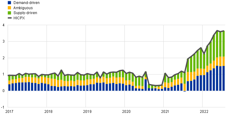
The decomposition suggests that the increase in euro area HICPX inflation starting in the third quarter of 2021 was initially mainly supply-driven, but the importance of demand factors has gradually increased over time. Over recent months, supply and demand factors have played broadly similar roles in HICPX inflation (Chart B). Robustness checks using HICPX series at constant tax rates (to account, for example, for the temporary cut in VAT in Germany in the second half of 2020) lead to similar results.
Chart B
HICPX inflation – decomposition into supply and demand-driven factors
(annual percentage changes; percentage point contributions)

Sources: Eurostat and ECB staff calculations.
Notes: Seasonally adjusted data. Based on the approach developed by Adam Shapiro. HICPX inflation reflects the sum of demand-driven, supply-driven and ambiguous components, calculated as the trailing sum of the last 12 monthly contributions. While price data are available for August 2022, the latest observation is for July 2022 as the turnover series used as a proxy for activity are published with some delay.
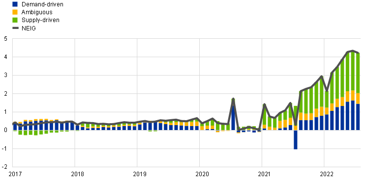
Looking at the main components of HICPX inflation, supply factors have played a somewhat bigger role in non-energy industrial goods (NEIG) inflation since early 2021 (Chart C). Changes in both demand and supply have strongly contributed to the increase in NEIG inflation since autumn 2021. Changes in supply did not play a significant role in NEIG inflation developments from 2017 to 2020, but they became the main driver of NEIG inflation in 2021, reflecting the effects of supply bottlenecks. Since late 2021, with the reopening of the economy, changes in demand are increasingly at play, but supply factors have remained dominant. Looking at individual components, components that contribute most to current NEIG inflation, such as motor cars and major household appliances, are classified as mainly supply-driven, while the rise in furniture prices, for example, is classified as mainly demand-driven.
Chart C
Decomposition of NEIG inflation
(annual percentage changes; percentage point contributions)

Sources: Eurostat and ECB staff calculations.
Notes: Seasonally adjusted data. Based on the approach developed by Adam Shapiro. NEIG inflation reflects the sum of demand-driven, supply-driven and ambiguous components, calculated as the trailing sum of the last 12 monthly contributions. While price data are available for August 2022, the latest observation is for July 2022 as the turnover series used as a proxy for activity are published with some delay.
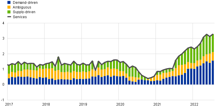
The strong increase in services inflation since mid-2021 has been driven by both demand and supply factors, with demand factors being more important for services inflation than for NEIG inflation (Chart D). Supply and demand factors tended to contribute broadly similarly to services inflation from 2017 to 2020, when services inflation was quite stable in the euro area. The strong increase in services inflation from mid-2021 onwards was initially driven mainly by supply factors. Contributions from predominantly supply-driven components increased strongly in the second half of 2021, but then remained relatively stable until mid-2022. The role of demand factors in services inflation began to increase only in the last months of 2021 – with the intensification of reopening effects – and continued to increase until mid-2022. More recently the contributions of predominantly demand-driven components to services inflation have outweighed those of predominantly supply-driven components. Zooming in on components, under the disaggregated approach inflation for package holidays and air flights is found to be mainly demand-driven, while inflation for maintenance and repair services for dwellings is found to be predominantly supply-driven.
Chart D
Decomposition of services inflation
(annual percentage changes; percentage point contributions)

Sources: Eurostat and ECB staff calculations.
Notes: Seasonally adjusted data. Based on the approach developed by Adam Shapiro. Services inflation reflects the sum of demand-driven, supply-driven and ambiguous components, calculated as the trailing sum of the last 12 monthly contributions. While price data are available for August 2022, the latest observation is for July 2022 as the turnover series used as a proxy for activity are published with some delay.
The disaggregated approach to the decomposition of HICPX inflation helps to show the role of supply and demand factors in underlying inflation, but there are important caveats with this method. The key advantage of this approach is that it allows each HICPX component to be classified as predominantly demand-driven or predominantly supply-driven. This makes the results very transparent and allows them to be cross-checked against other evidence available for inflation developments for various components. This transparency is especially valuable in the current environment of very high uncertainty resulting from the effects of the pandemic and the war in Ukraine on changes in activity and prices. But some caveats need to be kept in mind. First, there are different options for matching data on prices and activity, which is complicated by the fact that separate turnover series are not available for every HICPX component (this requires some HICPX components to be matched to the same turnover series, particularly in the case of NEIG inflation). Second, the disaggregated approach cannot quantify how large the supply and demand contributions are for each component. This could introduce a bias if, for example, the role of supply factors for components classified as predominantly demand-driven is on average much larger than the role of demand factors for components classified as predominantly supply-driven. In addition, developments in quantities and prices have clearly been exceptional since the start of the pandemic and have been influenced by many special factors, making it more difficult to build a reliable model as a basis for classification based on the signs of its errors.
We are grateful to Adam Shapiro for his guidance and support in applying his approach to the euro area and to Omiros Kouvavas for his help in matching data on prices and activity for the euro area.
See Shapiro, A.H., “How Much Do Supply and Demand Drive Inflation?”, FRBSF Economic Letter, No 2022-15, Federal Reserve Bank of San Francisco, 21 June 2022; and Shapiro, A.H., “Decomposing Supply and Demand Driven Inflation”, Working Papers, No 2022-18, Federal Reserve Bank of San Francisco, September 2022.
Ten-year-window rolling regressions (starting in January 2002) are run which include monthly data on both activity and prices and 12 lags in a standard two-equation vector autoregression (VAR) model. If the residuals for quantities and prices in the final months of each window have the same sign, that component is labelled as “demand-driven”, whereas, if they have opposite signs, it is identified as “supply-driven”. If the residual for either the price or the quantity series is statistically indistinguishable from zero, the category is labelled as “ambiguous” for that month.
To identify these ambiguous cases, we follow Shapiro’s baseline approach and label the middle 20% of the residuals in the respective regression sample distributions as ambiguous. This means that we compare the final month’s residuals discussed above with all residuals obtained in that window and assess whether or not it is in the middle 20% of the distribution. In the baseline specification, post-2020 residuals in the sample are excluded when running this test. However, a robustness test shows that the ambiguous component increases only slightly when post-2020 results are also included and that the overall results are not substantially affected.
Following Shapiro, the year-on-year supply and demand-driven contributions are then defined as the running total of the last 12 monthly supply and demand-driven contributions.
Based on the four-digit COICOP classification.
Turnover data are provided by Eurostat as part of short-term business statistics (see “Short-term business statistics introduced”, Statistics Explained, Eurostat). Data on services turnover (sts_setu_q) and retail trade turnover (sts_trtu_q) are used. The turnover series for services are deflated by the HICP in order to analyse turnover developments in real terms. Retail trade turnover series are already available deflated and non-deflated.
One caveat is that, for this analysis, the 72 HICPX components can only be matched to 45 turnover series (that are available in a sufficiently timely manner). Hence, some HICPX series (especially in NEIG) are matched to the same turnover series. The same matching approach is also used in, for example, “Consumption patterns and inflation measurement issues during the COVID-19 pandemic”, Economic Bulletin, Issue 7, ECB, 2020.


